

Lower Your Minimum Detectable Effect Without More Traffic
The minimum detectable effect (MDE) is the smallest true change your experiment can reliably catch at your chosen power and significance level, given the sample you actually have. If the smallest lift your business cares about is smaller than your MDE, you’re not testing. You’re guessing with extra steps, and no amount of clever analysis fixes that after the fact.
TL;DR:
- If your business needs to detect effects smaller than your current MDE, increasing traffic or rerunning the test may be necessary, as MDE scales with the inverse square root of sample size.
- Adjusting alpha to 0.01 or increasing power from 0.80 to 0.90 raises the MDE, meaning detecting smaller effects becomes more difficult without additional sample or longer duration.
- Incorporating variance reduction techniques like CUPED, stratification, or within-subject designs can lower MDE without extra traffic, making tests more sensitive.
- Always report the MDE alongside null results to clarify what size effects the test could reliably detect, avoiding misinterpretation of non-significant outcomes.
Table of Contents
- What Is MDE? A Formal Definition and Why It Matters
- How Do Power, Alpha, and Sample Size Determine MDE?
- Calculating MDE: Formulas and Worked Examples
- How to Choose an MDE That Reflects Business Impact
- Practical Levers to Lower MDE Without Increasing Sample
- How to Report MDE and Interpret Null Results
- Best Practices and Common Pitfalls in MDE Planning
- Applying MDE to Ad Creative and Marketing Tests
- Why Most Teams Get MDE Backwards
- Sources
- FAQ
What Is MDE? A Formal Definition and Why It Matters
MDE is a design number, not a result. It tells you, before you launch anything, the smallest true effect your test is built to catch given your sample size, your significance threshold (alpha), and your statistical power. This is the core idea behind power calculations as outlined by the World Bank’s DIME research group, which treats MDE as an output of the same math that determines sample size, not a separate guess.
Here’s where people get tripped up. MDE is not the effect you expect to see, and it’s not the effect you actually observed once the test wrapped. Those are three different numbers:
- MDE: the smallest effect your test design is sensitive enough to detect
- Expected effect: your hypothesis or prior belief about the true lift
- Observed effect: whatever the data happened to show once the test ran
Confusing the observed effect with MDE is how teams end up misreading null results. If your MDE is 5 percentage points and your test shows a 2 point lift that isn’t statistically significant, that doesn’t mean there’s no effect. It means your test was never built to see anything smaller than 5 points, so a 2 point signal was invisible from the start. Spotify’s Confidence documentation frames this well: MDE describes what your study could detect, not what’s actually happening in the world.
Think of MDE like the resolution on a camera. A phone camera captures a sunset fine but misses individual grains of sand on the beach. Your experiment is the same. Give it enough traffic and time, and it resolves a 1% lift. Starve it of sample, and it can only resolve something closer to a 15% lift, meaning anything smaller passes right through undetected. That’s not a flaw in your statistics. It’s a limitation you set the moment you decided how much traffic and how many days to commit.
How Do Power, Alpha, and Sample Size Determine MDE?
Four numbers govern every experiment: sample size, statistical power, significance level (alpha), and MDE. Fix any three, and the fourth is locked in. That’s not a rule of thumb. It’s algebra. Most calculators (and most experimentation platforms) let you solve for whichever one you’re missing, but the relationship never changes.
The one worth internalizing is how MDE scales with sample size. MDE is proportional to 1 divided by the square root of your sample size (n). MetricGate’s breakdown of the formula puts a clean number on this: doubling your sample only shrinks MDE by a factor of about 1.41, not 2.
Statistic callout: To cut your MDE in half, you need roughly four times the sample. That square root relationship is the single most underappreciated fact in experiment planning. Teams routinely double their traffic allocation expecting to double their sensitivity, then get confused when the improvement feels marginal.
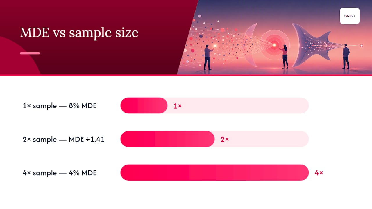
That nonlinearity has real consequences for planning. If your current MDE is 8% relative lift and you need to get down to 4% to detect something the business cares about, you’re not looking at 2x the runtime. You’re looking at roughly 4x. On a test that would’ve taken two weeks, that’s eight weeks, which changes the conversation with stakeholders from “let’s extend the test” to “let’s rethink the design.”
Alpha and power move MDE in the same direction, just less dramatically. Tightening alpha from 0.05 to 0.01 (fewer false positives, but harder to reach) raises your MDE for the same sample size, because you need a bigger signal to clear a stricter bar. Raising power from 0.80 to 0.90 (fewer missed true effects) does the same thing, since higher power demands more evidence before it commits to a conclusion.
The World Bank’s DIME guidance treats alpha = 0.05 and power = 0.80 as reasonable defaults, and most commercial testing tools ship with those baked in. But defaults aren’t laws. If a false positive would mean shipping a broken checkout flow to your entire customer base, tightening alpha to 0.01 is the more defensible choice even though it costs you sensitivity. If missing a true winner is the bigger risk (say, in early-stage growth experiments where volume is cheap), pushing power to 0.90 might be worth the extra sample.
Calculating MDE: Formulas and Worked Examples
The math behind MDE is an inversion of the standard power calculation. Instead of solving for sample size given a target effect, you solve for effect size given a fixed sample. Here’s how that plays out for the two most common test types.
Two-Proportion Tests (Conversion Rate Experiments)
For a two-proportion z-test, comparing conversion rates between a control and a variant, the MDE formula is:
MDE = (z₁₋α/2 + z₁₋β) × √(2p(1 − p) / n)
Where p is your baseline conversion rate, n is the sample size per group, and the z-values come from your chosen alpha and power. At the standard alpha of 0.05 (two-sided) and power of 0.80, z₁₋α/2 ≈ 1.96 and z₁₋β ≈ 0.84.
Worked example: Say your landing page converts at 10% (p = 0.10), and you’re planning to run 10,000 visitors per group.
- Calculate the standard error component: √(2 × 0.10 × 0.90 / 10,000) = √(0.000018) ≈ 0.00424
- Multiply by the combined z-score: (1.96 + 0.84) × 0.00424 = 2.80 × 0.00424 ≈ 0.0119
- Convert to a readable figure: your MDE is roughly 1.19 percentage points, meaning the test can detect a jump from 10% to about 11.19% conversion, but nothing smaller
This distinction matters more than most people realize, and Statistics.tools’ explanation of MDE calculation makes the point directly: the same relative lift means wildly different things depending on your starting baseline. Always report both figures, and never quote relative lift without stating the baseline it’s built on.
Two-Sample Means (Revenue, Time-on-Page, AOV)
When you’re comparing averages instead of proportions (average order value, session duration, revenue per user), the formula shifts slightly:
MDE = (z₁₋α/2 + z₁₋β) × σ × √(1/n₁ + 1/n₂)
Here σ is the standard deviation of your metric, and n₁, n₂ are your group sizes. MetricGate’s formula reference frames this in terms of Cohen’s d, a standardized effect size that expresses the difference in standard deviation units rather than raw units. To convert Cohen’s d back into something reportable, multiply d by your metric’s standard deviation. A Cohen’s d of 0.2 on an AOV metric with a standard deviation of $25 becomes a detectable absolute difference of $5.
| Test type | Formula core | What you need to know |
|---|---|---|
| Two-proportion (conversion) | (z₁₋α/2 + z₁₋β) × √(2p(1−p)/n) | Baseline rate, sample size per group |
| Two-mean (revenue, time) | (z₁₋α/2 + z₁₋β) × σ × √(1/n₁ + 1/n₂) | Standard deviation, sample size per group |
| Cohen’s d (standardized) | d = effect / σ | Convert back to raw units by multiplying by σ |
You rarely need to run these by hand. R’s pwr package (pwr.2p.test for proportions, pwr.t.test for means) and Python’s statsmodels.stats.power module handle the algebra, and most experimentation platforms surface an MDE estimate directly in the setup screen.
Pro Tip: Always run the calculation twice, once solving for MDE given your planned sample and once solving for sample size given the smallest MDE you’d act on. If the two numbers don’t match your actual traffic and timeline, you’ve found the gap before you’ve wasted a single day of test traffic.
How to Choose an MDE That Reflects Business Impact
The mistake most teams make is treating MDE as a purely statistical decision. It isn’t. MDE should start with a dollar or user-impact question: what’s the smallest lift that would actually change a decision?
Start by converting your KPI into revenue terms. If your fixed costs to build and ship the winning variant are $15,000, even a 0.5 point lift clears the bar. A test built to detect only 3+ point moves would blind you to a change worth tens of thousands of dollars a year.
Once you know the smallest effect worth detecting, run it against your actual traffic and timeline using a quick checklist:
- Does your available sample, run over a reasonable window (2 to 4 weeks is typical), get you an MDE at or below your business-meaningful threshold?
- If not, can you extend the test duration without the results going stale (seasonality, promotions, algorithm changes)?
- If extending isn’t realistic, can you raise your MDE and accept that only larger effects will register, while smaller wins go undetected?
- Is there a design change (see the variance-reduction section below) that gets you a smaller MDE without more traffic at all?
Optimizely’s guidance on using MDE for experiment design makes this trade-off explicit: MDE is the tool that turns “how long should this test run” into a business conversation instead of a statistics lecture.
Pro Tip: When a low-traffic page can’t reach a meaningful MDE in any reasonable timeframe, that’s not a reason to run the test anyway and hope. It’s a signal to test something with a bigger expected effect, like a full redesign instead of a button color, since larger changes need less sample to detect.
Practical Levers to Lower MDE Without Increasing Sample
You don’t have to buy more traffic to sharpen your test’s sensitivity. Several design and analysis choices shrink variance directly, which lowers MDE at the same sample size.
- CUPED (Controlled-experiment Using Pre-Experiment Data): adjusts for a covariate measured before the test started, like a user’s historical conversion rate or past spend, stripping out variance that has nothing to do with the treatment itself.
- Blocking and stratification: grouping similar users (by device, geography, or existing engagement tier) before randomizing reduces the noise those differences would otherwise add to your comparison.
- Paired or within-subject designs: when feasible, comparing the same user’s behavior before and after exposure removes between-user variance entirely, which is often the biggest source of noise in the first place.
- Metric selection: a binary conversion metric is noisier than a continuous one built from more data points; aggregating revenue over a longer window, for example, often produces a tighter, more sensitive metric than daily conversion rate alone.
MetricGate’s discussion of variance reduction techniques points out that CUPED alone commonly cuts required sample size by 20 to 50%, depending on how predictive the covariate is. That’s not a universal number; a covariate with weak correlation to your outcome metric won’t help much. But a covariate like 30-day pre-period spend, when your outcome metric is post-period spend, is usually strong enough to matter.
Blocking carries a risk if you get too aggressive with it: the more strata you carve out, the smaller each becomes, and at some point you’re back to sample-size problems within each block. Use it where the underlying subgroups genuinely differ, not as a reflexive default.
How to Report MDE and Interpret Null Results
Every experiment write-up should state its MDE alongside the point estimate and confidence interval, not bury it in a methods appendix. A result reported as “no significant difference, MDE was 6.2 percentage points” tells leadership something a bare “not significant” never can: the test was only built to catch fairly large moves, and anything below that threshold remains genuinely unknown.
- Report MDE, the observed effect, and the confidence interval together, every time, whether the result is significant or not.
- Never compute or report “observed power,” meaning power calculated after the fact using the effect size you happened to measure; research from J-PAL on underpowered evaluations flags this as a common and misleading practice, since observed power is mathematically just a rescaling of your p-value and adds no new information.
- A non-significant result with a small MDE (say, 1 to 2 points) is meaningful evidence that no practically important effect exists.
- A non-significant result with a large MDE (10+ points) tells you almost nothing; the honest next step is redesign, not a shrug.
- Before rerunning a null test, ask whether you can lower variance (see the levers above) rather than just running the same design longer.
Best Practices and Common Pitfalls in MDE Planning
Most MDE mistakes trace back to a handful of habits, and they’re avoidable once you know to watch for them.
- Set your MDE before collecting any data, and write it down. Deciding after the fact what counts as a “meaningful” effect invites motivated reasoning once you’ve seen the numbers.
- Don’t peek at results and stop early when they look good. Ad hoc peeking inflates your false positive rate well beyond your stated alpha; Evan Miller’s analysis of sequential testing explains why informal monitoring breaks the guarantees your test was designed around, and shows how planned sequential methods let you check results early without that penalty.
- Correct for multiple comparisons when testing several variants or metrics at once, and default to two-sided tests unless you have a specific, pre-registered reason to expect a change in only one direction.
- Document your assumptions: the baseline rate, the variance estimate, and the sample size you used to calculate MDE, so a colleague (or your future self) can audit the number six months later.
Applying MDE to Ad Creative and Marketing Tests
Marketing tests live under the same math, with one added wrinkle: the cost of running a live A/B test in ad platforms isn’t just statistical, it’s ad spend. Every impression burned on a losing creative variant is money that didn’t buy a conversion.
Start by converting your conversion-lift MDE into a ROAS or revenue threshold, the same way you would for a landing page.
That’s where pretesting earns its keep. Running creative concepts through synthetic audience feedback before they ever touch live spend narrows your live-test field down to genuinely distinct finalists, which does two things: it reduces the number of variants competing for the same traffic pool (lowering your multiple-comparisons burden), and it screens out weak concepts that would have needed a huge MDE to distinguish from the control anyway.
A workable creative-testing workflow looks like this:
- Generate and pretest creative concepts against synthetic buyer personas to catch obvious misses before spending a dollar on live traffic.
- Narrow to two or three finalists that show a meaningfully different response pattern in pretesting, not five near-identical variants.
- Set your live A/B test’s MDE based on documented assumptions: baseline conversion rate, expected traffic over the test window, and the smallest ROAS improvement that would justify a creative swap.
- Run the live ad testing workflow with that MDE stated up front, not discovered after the results come in confusing.
Pretesting doesn’t replace the live test. It reduces how much your live test has to prove, which is exactly what shrinks your required sample and your timeline. POPJAM’s free ad testing tool and the reasoning in why pretesting creatives cuts costs both point at the same underlying math this article covers: fewer, sharper variants mean a smaller, more affordable MDE. For a deeper look at connecting data to creative decisions, data-driven ad testing for ROI and general conversion rate optimization practices cover adjacent ground worth reading alongside this workflow.
Why Most Teams Get MDE Backwards
Most guidance on this topic treats MDE as a calculator output: plug in baseline, alpha, power, get a number, move on. That’s backwards. The number should come from the business question first, the traffic constraint second, and the formula last.
The bigger blind spot is reporting. Teams that carefully calculate MDE before launch routinely forget to state it afterward, so a null result reads as “nothing happened” instead of “we could only see effects above X, and nothing that big showed up.” That distinction changes what a reasonable person does next, whether that’s walking away, rerunning with a sharper design, or accepting a smaller effect exists but isn’t worth chasing.
That single fact should shape every conversation about extending a test versus redesigning it, and it should shape how creative teams pretest before they ever touch live ad spend.
— Doruk
Sources
- Power Calculations | DIME Wiki - World Bank
- Use minimum detectable effect when you design an experiment - Optimizely Support
- Minimum Detectable Effect Explained | MetricGate
- Sequential AB testing discussion - Evan Miller
FAQ
How Do You Calculate Minimum Detectable Effect?
For proportions, MDE = (z₁₋α/2 + z₁₋β) × √(2p(1−p)/n), where p is your baseline rate and n is your sample size per group. For means, replace the proportion term with σ × √(1/n₁ + 1/n₂), using your metric’s standard deviation.
How Do You Calculate Minimum Detectable Change?
Minimum detectable change follows the same math as MDE. It’s the smallest true difference your test design can reliably catch given your sample size, chosen alpha, and target power, calculated by inverting the standard power formula.
Is a 0.3 Effect Size Good?
A Cohen’s d of 0.2 is generally considered a small effect, and 0.3 is around a small-to-medium effect. Whether it’s “good” depends entirely on context: in a landing page test, a 0.3 standardized effect might translate into a meaningful revenue lift, while in a clinical trial the same figure might be too small to justify treatment.
Is a P-Value Below 0.001 Considered Significant?
Yes, a p-value below 0.05 clears the standard significance threshold by a margin. A very small p-value indicates strong evidence against the null hypothesis, but it says nothing about whether the observed effect size is large enough to matter for your business.
What’s the Difference Between MDE and Statistical Power?
Power is the probability your test detects a true effect of a given size; MDE is the smallest effect size your test can detect at that power level. They’re two sides of the same power analysis, just solved for different unknowns.